Credit Risk Modeling
Note: Here I present a short report of the project. For a comprehensive report of this project including code scripts please refer to this page.
Overview:
Although the bank loans have benefits for bank however they are always under the risk of default of paying back. For reducing this risk the banks are interested in predicting the situation of returning the loan through evaluating applicant’s application form. Machine learning can help to reduce this risk by predicting the probability of default using different variables of applicants.
In this work I examine the logistic regression, decision tree and random forest to predicting the pay back status of loans on the German credit data set. The data is provided in two formats, one consists of 20 (7 numerical, 13 categorical) variables and the other one contains 24 numerical variables (for algorithms which strictly works with numerical variables). In the both formats the target variable (default) shows whether the loan applicant could make payment (0/NonDef) or not (1/Def). I divide the data to the test and training data sets. I will use the training set for training the algorithms and finding the most efficient model and keep the test data set unseen to check the real performance of the selected models.
I use R programming language with extra packages like rpart, rpart.plot, randomForest, caret, pROC, doMC, glm function with some other functions which designed in the code. I consider AUC (Area Under ROC) as a metric to check the efficiency of models on the training data set through repeated cross-validations. Apart from a demand for high accuracy, sensitivity and specificity of a model, a low value of the bad rate is also desired from the bank. The bad rate is defined as the ratio of false negative to the total actual negative examples. The low value of the bad rate shows the less number of actual positive default cases which are wrongly predicted as the non-default cases. This reduces the risk of loss for the bank. Although a low bad rate is desirable but it must along with a proper percentage of acceptance ratio of applicants. For this project I assume a maximum of 15% bad rate and minimum 60% acceptance ratio are reasonable and is the goal of a particular bank. Therefore my final target will be finding the best model which can satisfy these criteria.
Logistic Regression
I start with the most general model (fml0) includes 24 variables/predictors. Then I check the p-values of predictors (via the repeated Cross-Validation on training data set) and remove predictors which has the worst p-value (>0.05) to build another model. I repeat this procedure till the p-values of all coefficients are less than 0.05. A the end I obtain 17 logistic regression models. Then I calculate the average AUC value for each model (via the repeated CV). The below figure shows the average AUC values for 17 logistic regression models.
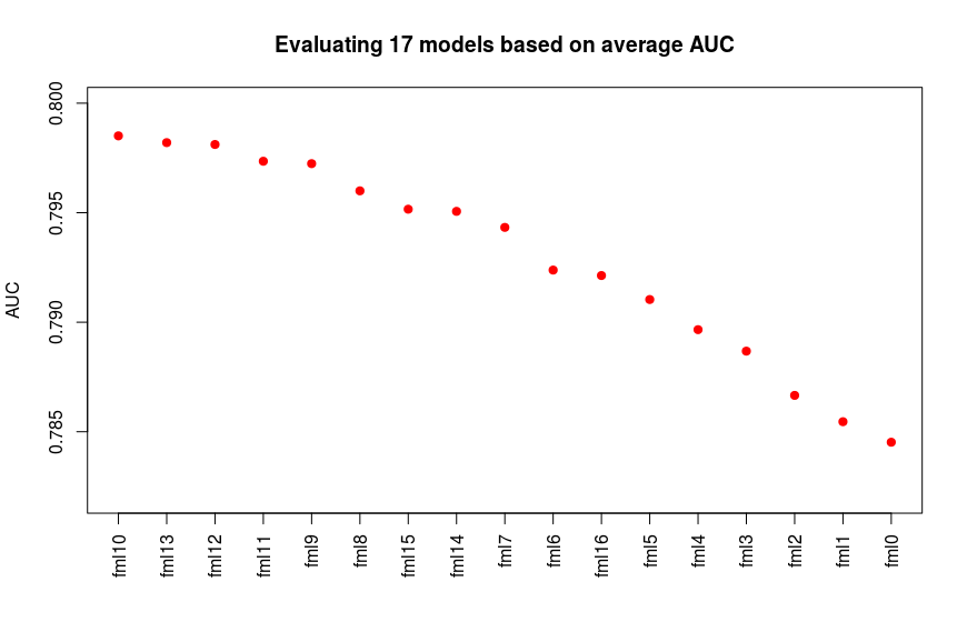
We can see the fml10, fml13, fml12 shows better AUC values. Considering the first four models which have the highest average AUC values and the fml0 as the most general model, I calculate the trend of bad rate of these 5 models based on acceptance ratio to select the best model wich satisfies our goal. The below figure illustrates average bad rates of the models calculated through repeated CV:
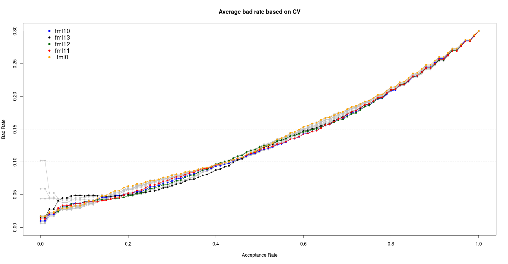
From the this plot we can see the fml10 and fml11 show the best performance between 10% to 15% bad rate range. Since the fml10 has already shown the better AUC value I select the fml10 as the best logistic model. It worth note that this model is selected based on the training data set. Its actual performance will be checked in the last section of this report on unseen test data set.
Decision Tree
First I construct the trees with different complexity parameter values and choose the proposed trees based on the minimum average cross-validate error. The results are plotted below:
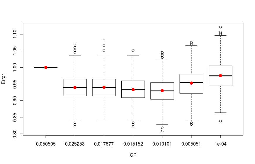
As we see the four trees with 0.01010101, 0.01515152, 0.01767677 and 0.02525253 complexity parameter values have the lowest errors.
Furthermore I examine the trees based on the average AUC on a grid of CP values via repeated CV on training data set:
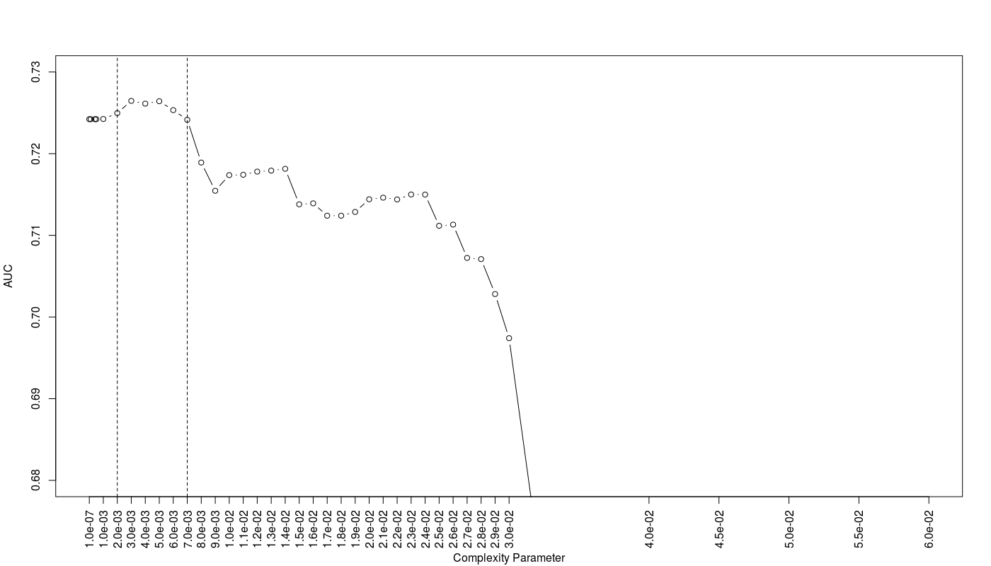
As we can see the trees with CP values between 0.002 to 0.007 show the best AUC efficiency.
Finally I have 10 proposed trees with different CP values. Following the similar procedure in evaluation of logistic models, I evaluate 10 proposed trees based on their bad rate:
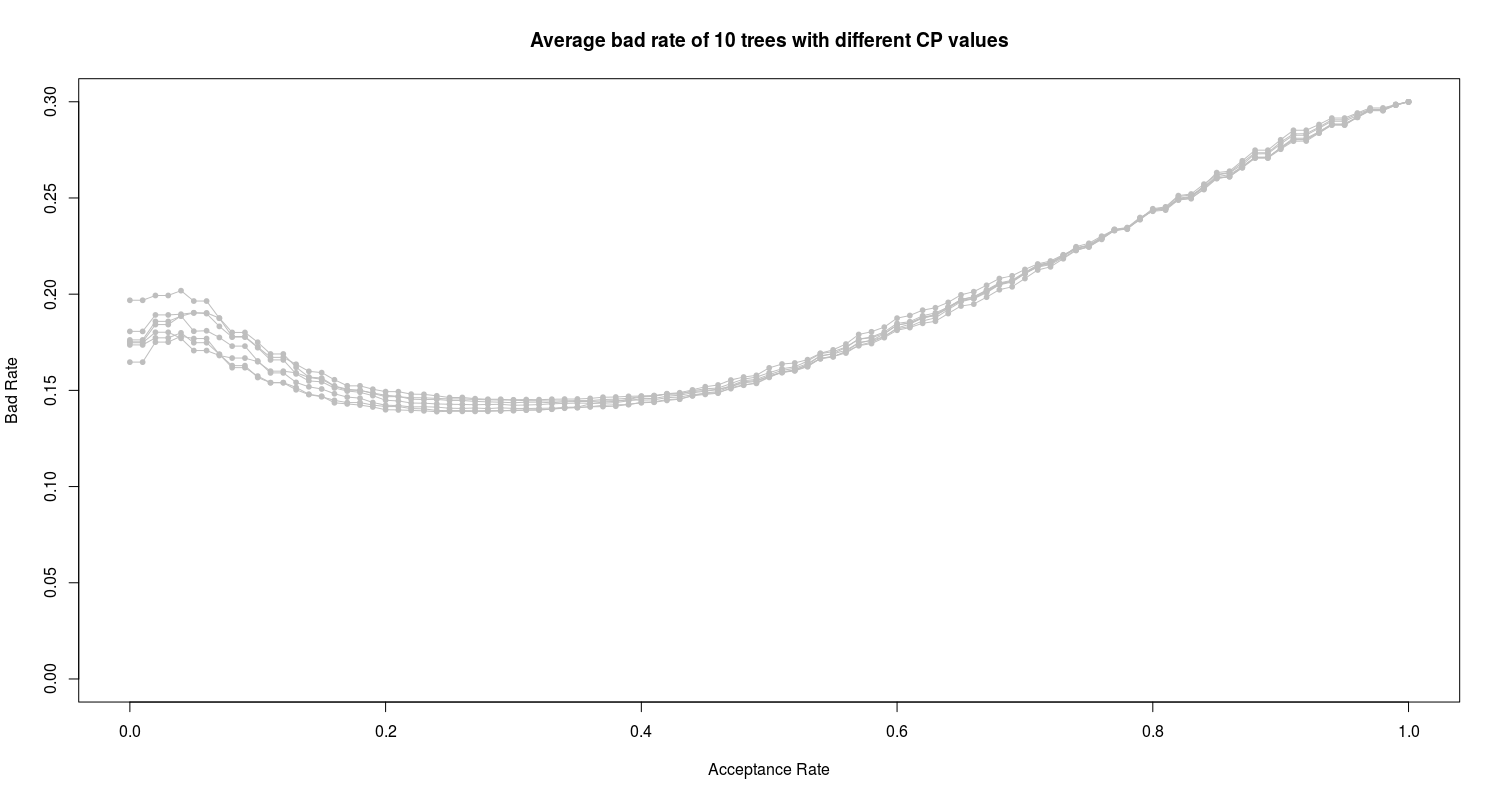
We can see the obvious high bad rate of all 10 proposed trees. In the next section I employ and train the random forest algorithm on the data.
Random Forest
I train random forest algorithm on training data set considering AUC for different mtry values (the number of features which are randomly selected at each split) in a repeated cross-validation method. The results are as below:
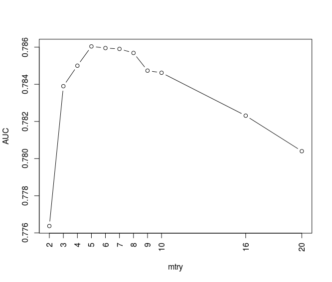
We can see the random forest models corresponding to mtry values between 3 to 10 show high AUC values. The below figure illustrates the bad rate trends of random forest models and compares with previous pruned tree models:
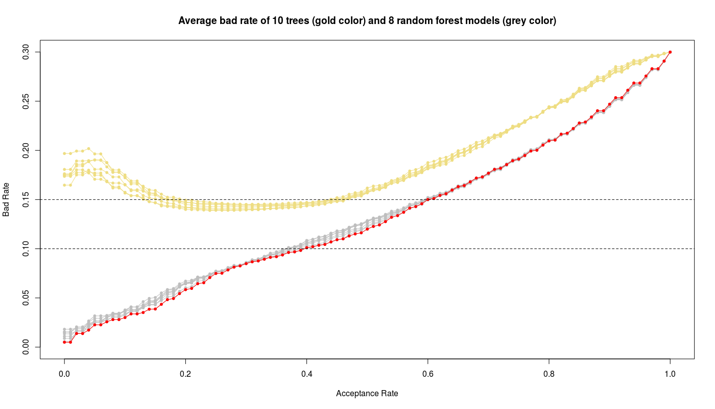
We see obviously the random forest models work better than tree models while the random forest with mtry=3 (red color) gives the best performance i.e. low bad rate with high acceptance rate.
Results of the final models
The fml10 logistic model and random forest with mtry=3 are the winners on the training data set. To see the real performance of both models I evaluate them on unseen test data set. The below figure illustrates the bad rate for both models:
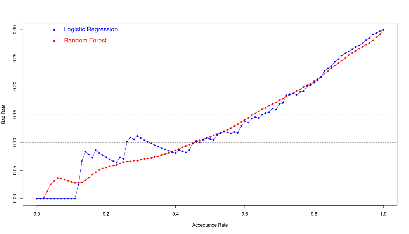
Assuming accepted maximum 15% bad rate we have:
acp_rate    cut_off   bad_rate    sens       spec        accu      kppa
Logistic Regression
65% 0.65 0.44823798 0.14932127 0.67647059 0.789915966 0.7558824 0.445187166

Random Forest
63% 0.63 0.4042546 0.151472427 0.68137255 0.764957983 0.7398824 0.418835806
We see the logistic regression and random forest show the similar efficiency however logistic regression shows slightly better performance at 15% bad rate. The 65% acceptance ratio at 15% bad rate with 76% accuracy and 0.44 kappa value is a good achievement for this model.