Credit Risk Modeling (details + scripts)
Data:
I use the German credit data set. The data is provided in two formats, one consists of 20 variables (7 numerical, 13 categorical) as below:
– Status of existing checking account
– Duration in month (numerical)
– Credit history
– Purpose
– Credit amount (numerical)
– Savings account/bonds
– Present employment since
– Installment rate in percentage of disposable income (numerical)
– Personal status and sex
– Other debtors / guarantors
– Present residence since (numerical)
– Property
– Age in years (numerical)
– Other installment plans
– Housing
– Number of existing credits at this bank (numerical)
– Job
– Number of people being liable to provide maintenance for (numerical)
– Telephone
– foreign worker
and the other one contains 24 numerical variables for algorithms which strictly works with numerical variables. In the both formats the default, target variable shows whether the loan applicant could make payment (0/NonDef) or not (1/Def).
After loading data sets as the data frames I check the distribution of variables and possibility of missing data. Fortunately there is no any abnormal behavior and missing data in both data sets. The summary of both formats of data sets are as following:
R> d.g <- read.table('./data/german.data')
R> colnames(d.g) <- c( 'account_balance',
                    'months_loan_duration',
                    'credit_history',
                    'purpose',
                    'credit_amount',
                    'savings_balance',
                    'employment_status',
                    'installment_rate',
                    'personal_status',
                    'other_debtors_guarantors',
                    'present_residence_years',
                    'property',
                    'age',
                    'other_installment',
                    'housing',
                    'number_credits_this_bank',
                    'job',
                    'number_dependents',
                    'phone',
                    'foreign_worker',
                     'default')

R> d.g$default <- factor(ifelse(d.g$default==1, 0, 1))
R> levels(d.g$default) <- c('Nondef', 'Def')

R> summary(d.g)
 account_balance   months_loan_duration   credit_history   purpose
 A11:274           Min. : 4.0             A30: 40          A43 :280
 A12:269           1st Qu.:12.0           A31: 49          A40 :234
 A13: 63           Median :18.0           A32:530          A42 :181
 A14:394           Mean :20.9             A33: 88          A41 :103
                   3rd Qu.:24.0           A34:293          A49 : 97
                   Max. :72.0                              A46 : 50
                                                        (Other): 55

 credit_amount   savings_balance   employment_status   installment_rate
 Min. : 250      A61:603           A71: 62             Min. :1.000
 1st Qu.: 1366   A62:103           A72:172             1st Qu.:2.000
 Median : 2320   A63: 63           A73:339             Median :3.000
 Mean : 3271     A64: 48           A74:174             Mean :2.973
 3rd Qu.: 3972   A65:183           A75:253             3rd Qu.:4.000
 Max. :18424                                           Max. :4.000

 personal_status   other_debtors_guarantors   present_residence_years   property
 A91: 50           A101:907                   Min. :1.000               A121:282
 A92:310           A102: 4                    1 1st Qu.:2.000           A122:232
 A93:548           A103: 52                   Median :3.000             A123:332
 A94: 92                                      Mean :2.845               A124:154
                                              3rd Qu.:4.000
                                              Max. :4.000

 age             other_installment   housing    number_credits_this_bank
 Min. :19.00     A141:139            A151:179   Min. :1.000
 1st Qu.:27.00   A142: 47            A152:713   1st Qu.:1.000
 Median :33.00   A143:814            A153:108   Median :1.000
 Mean :35.55                                    Mean :1.407
 3rd Qu.:42.00                                  3rd Qu.:2.000
 Max. :75.00                                    Max. :4.000

 job        number_dependents   phone      foreign_worker  default
 A171: 22   Min. :1.000         A191:596   A201:963        Nondef:700
 A172:200   1st Qu.:1.000       A192:404   A202: 37        Def :300
 A173:630   Median :1.000
 A174:148   Mean :1.155
            3rd Qu.:1.000
            Max. :2.000
and the numerical format:
R> d.g.num <- read.table('../data/german.data-numeric')
R> d.g.num$default <- factor(ifelse(d.g.num$V25==1, 0, 1))
R> d.g.num$V25 <- NULL

R> summary(d.g.num)
 V1             V2            V3             V4
 Min. :1.000    Min. : 4.0    Min. :0.000    Min. : 2.00
 1st Qu.:1.000  1st Qu.:12.0  1st Qu.:2.000  1st Qu.: 14.00
 Median :2.000  Median :18.0  Median :2.000  Median : 23.00
 Mean :2.577    Mean :20.9    Mean :2.545    Mean : 32.71
 3rd Qu.:4.000  3rd Qu.:24.0  3rd Qu.:4.000  3rd Qu.: 40.00
 Max. :4.000    Max. :72.0    Max. :4.000    Max. :184.00
 V5             V6             V7             V8
 Min. :1.000    Min. :1.000    Min. :1.000    Min. :1.000
 1st Qu.:1.000  1st Qu.:3.000  1st Qu.:2.000  1st Qu.:2.000
 Median :1.000  Median :3.000  Median :3.000  Median :3.000
 Mean :2.105    Mean :3.384    Mean :2.682    Mean :2.845
 3rd Qu.:3.000  3rd Qu.:5.000  3rd Qu.:3.000  3rd Qu.:4.000
 Max. :5.000    Max. :5.000    Max. :4.000    Max. :4.000

 V9             V10            V11            V12
 Min. :1.000    Min. :19.00    Min. :1.000    Min. :1.000
 1st Qu.:1.000  1st Qu.:27.00  1st Qu.:3.000  1st Qu.:1.000
 Median :2.000  Median :33.00  Median :3.000  Median :1.000
 Mean :2.358    Mean :35.55    Mean :2.675    Mean :1.407
 3rd Qu.:3.000  3rd Qu.:42.00  3rd Qu.:3.000  3rd Qu.:2.000
 Max. :4.000    Max. :75.00    Max. :3.000    Max. :4.000

 V13            V14            V15            V16
 Min. :1.000    Min. :1.000    Min. :1.000    Min. :0.000
 1st Qu.:1.000  1st Qu.:1.000  1st Qu.:1.000  1st Qu.:0.000
 Median :1.000  Median :1.000  Median :1.000  Median :0.000
 Mean :1.155    Mean :1.404    Mean :1.037    Mean :0.234
 3rd Qu.:1.000  3rd Qu.:2.000  3rd Qu.:1.000  3rd Qu.:0.000
 Max. :2.000    Max. :2.000    Max. :2.000    Max. :1.000

 V17            V18            V19            V20
 Min. :0.000    Min. :0.000    Min. :0.000    Min. :0.000
 1st Qu.:0.000  1st Qu.:1.000  1st Qu.:0.000  1st Qu.:0.000
 Median :0.000  Median :1.000  Median :0.000  Median :0.000
 Mean :0.103    Mean :0.907    Mean :0.041    Mean :0.179
 3rd Qu.:0.000  3rd Qu.:1.000  3rd Qu.:0.000  3rd Qu.:0.000
 Max. :1.000    Max. :1.000    Max. :1.000    Max. :1.000

 V21            V22            V23          V24            default
 Min. :0.000    Min. :0.000    Min. :0.0    Min. :0.00     0:700
 1st Qu.:0.000  1st Qu.:0.000  1st Qu.:0.0  1st Qu.:0.00   1:300
 Median :1.000  Median :0.000  Median :0.0  Median :1.00
 Mean :0.713    Mean :0.022    Mean :0.2    Mean :0.63
 3rd Qu.:1.000  3rd Qu.:0.000  3rd Qu.:0.0  3rd Qu.:1.00
 Max. :1.000    Max. :1.000    Max. :1.0    Max. :1.00
Methodology
I will apply logistic regression, decision tree and random forest on these data sets and evaluate their efficiency based on AUC (Area Under ROC), Kappa statistics and Bad Rate. Finally I will propose the best model which shows the best efficiency on the training data set.
1- Logistic Regression
First I divide the data to the test and training data sets. For this purpose I employ createDataPartition function from caret package to obtain the stratified random samples of the data. I will use the training set for training the algorithm and finding the most efficient model and keep the test data set to check the real performance of the selected model on an unseen data set.
R> prop.table(table(d.g.num$default))
0   1
0.7 0.3

R> library(caret)
R> in_train <- createDataPartition(d.g.num$default, p = 0.66, list = FALSE)
R> train_set <- d.g.num[in_train,]
R> test_set <- d.g.num[-in_train,]

R> prop.table(table(train_set$default))
0   1
0.7 0.3

R> prop.table(table(test_set$default))
0   1
0.7 0.3
I start by the most general model which includes all variables then construct the next model by omitting the predictor which has the worst p-value. Since the p-values of predictors have high dependency to training data set I calculate the average p-values through cross-validation in training data set. The pvalue.coef function return the p-values of coefficients of a given model.
R> pvalue.coef <- function(mdl)
+ {
+ dum <- summary(mdl)$coefficients
+ dum <- dum[,'Pr(>|z|)']
+ return(dum)
+ }
The eval_model_nonimpvar function with using cv_nonimpvar function calculates and plots the boxplot of p-values of coefficients through a repeated (100 times) 10-fold cross-validation for the given formula fml of the model.
R> cv_nonimpvar <- function(fml, folds)
+ {
+  rs <- lapply(folds, function(x)
+                                  {
+                                    train_set_train <- train_set[-x, ]
+                                    mdl <- glm(formula = fml, family = binomial(link=logit), data = train_set_train)
+                                    nonimpvar <- pvalue.coef(mdl)
+                                    return(nonimpvar)
+                                  })
+  vars_name <- all.vars(fml[[3]])
+  rs_matrix <- matrix(unlist(rs), nrow=length(vars_name)+1 )
+  colnames(rs_matrix) <- c(paste0('Fold0',1:9),'Fold10')
+  rownames(rs_matrix) <- c('Intercept', vars_name)
+  return(rs_matrix)
+ }
R> n.cv <- 100
R> eval_model_nonimpvar <- function(fml)
+                                      {
+                                       t.mat <- NULL
+                                       for (i in 1:n.cv)
+                                                       {
+                                                        folds.new <- createFolds(train_set$default, k = 10)
+                                                        cv_var_op <- cv_nonimpvar(fml, folds.new)
+                                                        t.mat <- cbind(t.mat, cv_var_op)
+                                                       }

+ dum <- apply(t.mat, 1, mean)
+ id <- order(dum, decreasing = T)
+ boxplot(t(t.mat[id,]), las=2, main=fml, ylim=c(0,.2))
+ points(dum[id], pch=20, cex=1, col='red')
+ return(t.mat)
+}
Applying for the most general model:
fml0 <- default ~ V1+V2+V3+V4+V5+V6+V7+V8+V9+V10+V11+V12+V13+V14+V15+V16+V17+V18+V19+V20+V21+V22+V23+V24
nonimpvar0.mat <- eval_model_nonimpvar(fml0)
I obtain the below results:
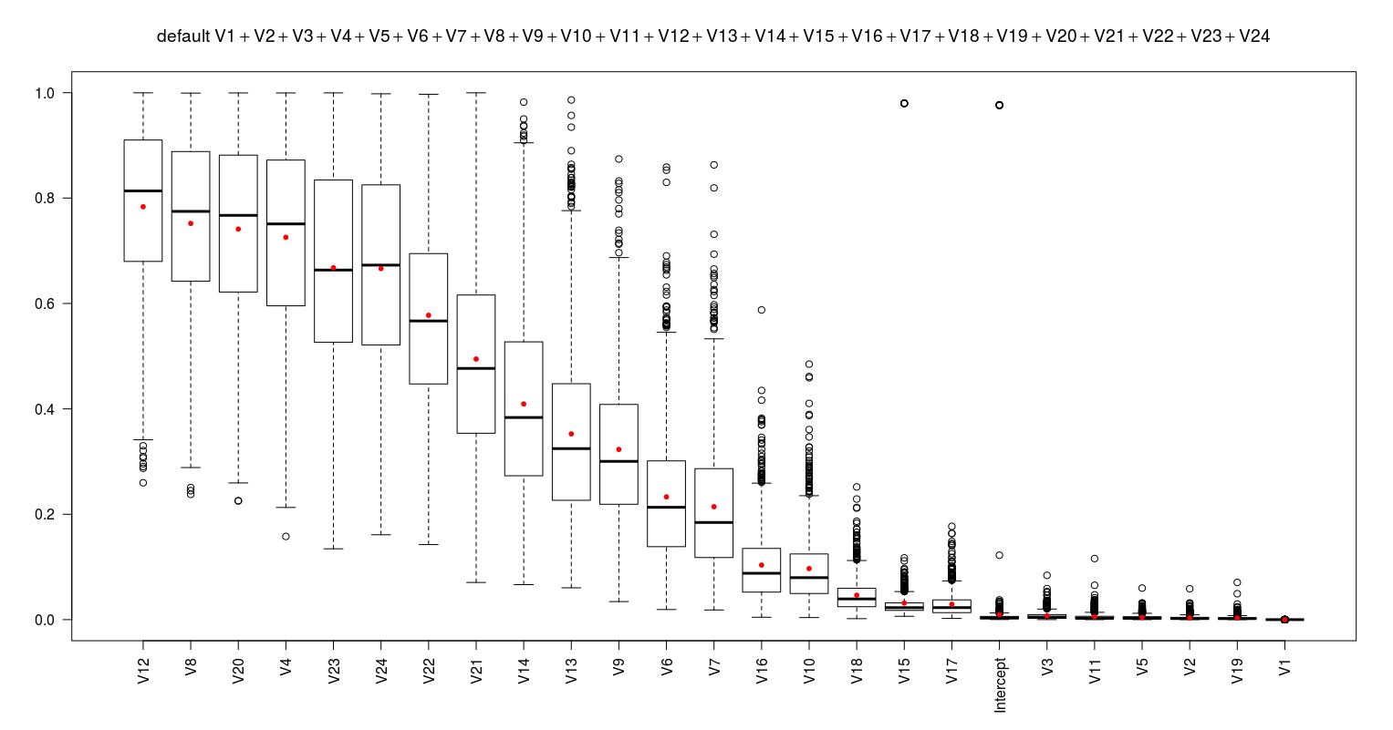
These results suggest to remove the V12 to form a better model (fml1). After removing it I repeat the same procedure to obtain the next worst predictor. I continue this procedure till all the predictors show the average p-value less than 0.05. This proposes 16 models (as below) which are simpler than the fml0.
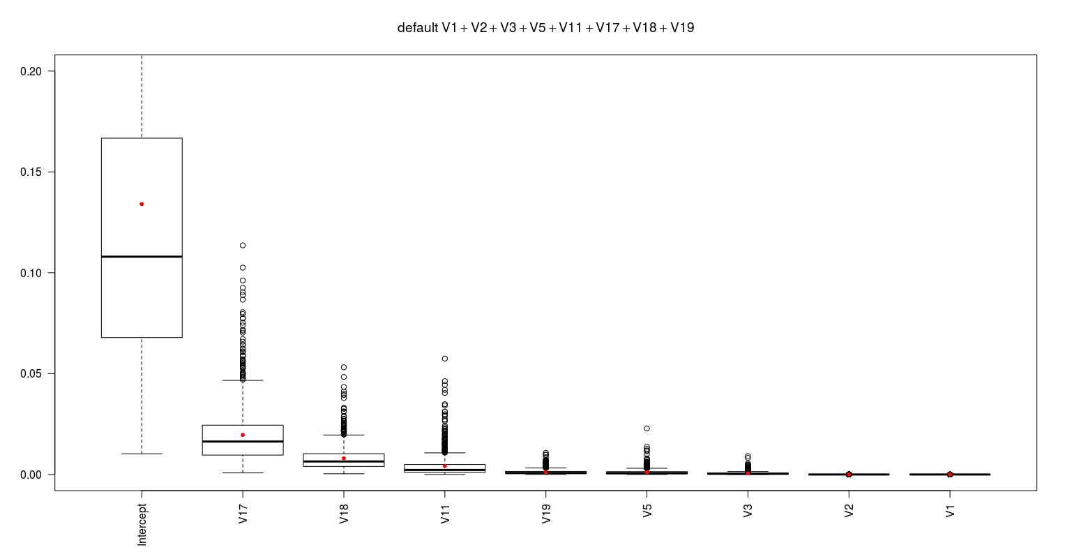
#--------------------------------------------------------------------------------------------------------
fml1 <- default ~ V1+V2+V3+V4+V5+V6+V7+V8+V9+V10+V11+V13+V14+V15+V16+V17+V18+V19+V20+V21+V22+V23+V24 #12
nonimpvar1.mat <- eval_model_nonimpvar(fml1)
#--------------------------------------------------------------------------------------------------------
fml2 <- default ~ V1+V2+V3+V4+V5+V6+V7+V9+V10+V11+V13+V14+V15+V16+V17+V18+V19+V20+V21+V22+V23+V24 #12, 8
nonimpvar2.mat <- eval_model_nonimpvar(fml2)
#--------------------------------------------------------------------------------------------------------
fml3 <- default ~ V1+V2+V3+V4+V5+V6+V7+V9+V10+V11+V13+V14+V15+V16+V17+V18+V19+V21+V22+V23+V24 #12, 8, 20
nonimpvar3.mat <- eval_model_nonimpvar(fml3)
#--------------------------------------------------------------------------------------------------------
fml4 <- default ~ V1+V2+V3+V5+V6+V7+V9+V10+V11+V13+V14+V15+V16+V17+V18+V19+V21+V22+V23+V24 #12, 8, 20, 4
nonimpvar4.mat <- eval_model_nonimpvar(fml4)
#--------------------------------------------------------------------------------------------------------
fml5 <- default ~ V1+V2+V3+V5+V6+V7+V9+V10+V11+V13+V14+V15+V16+V17+V18+V19+V21+V22+V24 #12, 8, 20, 4, 23
nonimpvar5.mat <- eval_model_nonimpvar(fml5)
#--------------------------------------------------------------------------------------------------------
fml6 <- default ~ V1+V2+V3+V5+V6+V7+V9+V10+V11+V13+V14+V15+V16+V17+V18+V19+V21+V22 #12, 8, 20, 4, 23, 24
nonimpvar6.mat <- eval_model_nonimpvar(fml6)
#--------------------------------------------------------------------------------------------------------
fml7 <- default ~ V1+V2+V3+V5+V6+V7+V9+V10+V11+V13+V14+V15+V16+V17+V18+V19+V21 #12, 8, 20, 4, 23, 24, 22
nonimpvar7.mat <- eval_model_nonimpvar(fml7)
#--------------------------------------------------------------------------------------------------------
fml8 <- default ~ V1+V2+V3+V5+V6+V7+V9+V10+V11+V13+V15+V16+V17+V18+V19+V21 #12, 8, 20, 4, 23, 24, 22, 14
nonimpvar8.mat <- eval_model_nonimpvar(fml8)
#--------------------------------------------------------------------------------------------------------
fml9 <- default ~ V1+V2+V3+V5+V6+V7+V9+V10+V11+V13+V15+V16+V17+V18+V19 #12, 8, 20, 4, 23, 24, 22, 14, 21
nonimpvar9.mat <- eval_model_nonimpvar(fml9)
#--------------------------------------------------------------------------------------------------------
fml10 <- default ~ V1+V2+V3+V5+V6+V7+V9+V10+V11+V15+V16+V17+V18+V19 #12, 8, 20, 4, 23, 24, 22, 14, 21, 13
nonimpvar10.mat <- eval_model_nonimpvar(fml10)
#--------------------------------------------------------------------------------------------------------
fml11 <- default ~ V1+V2+V3+V5+V7+V9+V10+V11+V15+V16+V17+V18+V19 #12, 8, 20, 4, 23, 24, 22, 14, 21, 13, 6
nonimpvar11.mat <- eval_model_nonimpvar(fml11)
#--------------------------------------------------------------------------------------------------------
fml12 <- default ~ V1+V2+V3+V5+V9+V10+V11+V15+V16+V17+V18+V19 #12, 8, 20, 4, 23, 24, 22, 14, 21, 13, 6, 7
nonimpvar12.mat <- eval_model_nonimpvar(fml12)
#--------------------------------------------------------------------------------------------------------
fml13 <- default ~ V1+V2+V3+V5+V10+V11+V15+V16+V17+V18+V19 #12, 8, 20, 4, 23, 24, 22, 14, 21, 13, 6, 7, 9
nonimpvar13.mat <- eval_model_nonimpvar(fml13)
#--------------------------------------------------------------------------------------------------------
fml14 <- default ~ V1+V2+V3+V5+V11+V15+V16+V17+V18+V19 #12, 8, 20, 4, 23, 24, 22, 14, 21, 13, 6, 7, 9, 10
nonimpvar14.mat <- eval_model_nonimpvar(fml14)
#--------------------------------------------------------------------------------------------------------
fml15 <- default ~ V1+V2+V3+V5+V11+V15+V17+V18+V19 #12, 8, 20, 4, 23, 24, 22, 14, 21, 13, 6, 7, 9, 10, 16
nonimpvar15.mat <- eval_model_nonimpvar(fml15)
#--------------------------------------------------------------------------------------------------------
fml16 <- default ~ V1+V2+V3+V5+V11+V17+V18+V19 #12, 8, 20, 4, 23, 24, 22, 14, 21, 13, 6, 7, 9, 10, 16, 15
nonimpvar16.mat <- eval_model_nonimpvar(fml16)
#--------------------------------------------------------------------------------------------------------
The following figure shows the p-values of the coefficient of the last model (fml16).
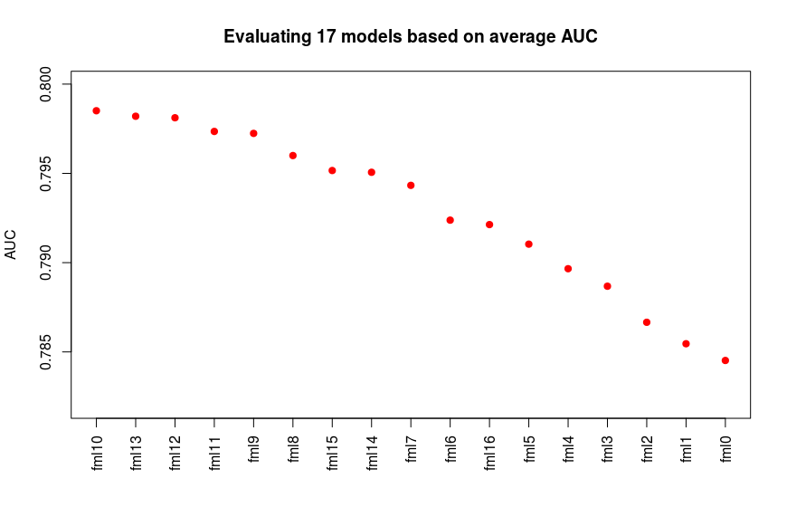
Having 17 models I evaluate them based on AUC (Area Under ROC). I use pROC and caret packages to calculate average AUC for models using repeated (100 times) 10-fold cross-validation.
library(pROC)

cv_auc_function <- function(fml, folds)
{
  auc_r <- lapply(folds, function(x)
  {
    train_set_train 	<- train_set[-x, ]
    train_set_test 	<- train_set[x, ]

    mdl 	      <- glm(formula = fml, family = binomial(link=logit), data = train_set_train)
    pred 	      <- predict(mdl, newdata = train_set_test, type = 'response')
    dum.roc     <- roc(train_set_test$default, pred)

    as.vector(auc(dum.roc))

  })
  return(unlist(auc_r))
  # Output is a vector like:
  # Fold01    Fold02    Fold03    Fold04    Fold05    Fold06    Fold07    Fold08    Fold09    Fold10
  # 0.7456522 0.8832952 0.8478261 0.8836957 0.7652174 0.6904255 0.7425532 0.7356979 0.7804348 0.7739130
}
#.............................................
fml_vec <- paste0('fml', 0:16)
auc_matrix_cv <- NULL
for (i in fml_vec)
{
  fml <- get(i)

  t.vec <- NULL
  for ( j in 1:n.cv)
  {
    folds.new <- createFolds(train_set$default, k = 10)
    dum <- cv_auc_function(fml, folds.new)
    t.vec <- c(t.vec, dum)
  }
  auc_matrix_cv <- cbind(auc_matrix_cv, t.vec)
}
colnames(auc_matrix_cv) <- fml_vec
auc_means <- apply(auc_matrix_cv, 2, mean)
id <-  order(auc_means, decreasing = T)

plot(auc_means[id], xaxt='n', xlab='', ylim=c(0.782, 0.8), pch=20,cex=1.5, col='red', ylab='AUC', main='Evaluating all 16 models based on AUC via CV') #CV2.png
axis(1,at=1:17,labels=names(auc_means[id]), las=2)
As we see in the results in following plot the fml10 shows the best average AUC while followed by fml13, fml12 and fml11 models.
For a bank apart from a demand for high accuracy, sensitivity and specificity of a model, a low value of the bad rate is also desired. The bad rate is defined as the ratio of false negative to the total actual negative examples. The low value of bad rate shows the less number of actual positive default cases which are wrongly predicted as the non-default cases. This reduces the risk of loss for the bank. Although a low bad rate is desirable but it must along with a proper percentage of acceptance ratio of applicants. For this project I assume a maximum of 15% bad rate and minimum 60% acceptance ratio are reasonable for a particular bank. Therefore I try to find the best model which can satisfy these criteria.
The following br.se.ac function calculate the bad rate, sensitivity, specificity, accuracy and kappa statistics in the range of 0% to 100% acceptance ratio for a particular model.
#------br.se.ac function--------------------------------------------------

br.se.ac <- function(actl_class, pred_prob)
{
  acp_rate <- seq(0,1,by=0.01)
  cut_off  <- NULL
  bad_rate <- NULL
  sens     <- NULL
  spec     <- NULL
  accu     <- NULL
  kppa     <- NULL
  for (i in 1:length(acp_rate))
  {
    cutoff <- quantile(pred_prob, acp_rate[i])
    pred_class <- ifelse(pred_prob> cutoff, 1, 0)
    pred_class <- factor(pred_class, levels=levels(actl_class))

    cont_table <- table(actl_class, pred_class)

    TN <- cont_table[1,1]
    FP <- cont_table[1,2]
    FN <- cont_table[2,1]
    TP <- cont_table[2,2]

    br <- FN/(FN+TN)
    se <- TP/(TP+FN)
    sp <- TN/(TN+FP)
    ac <- (TN+TP)/(TN+FP+FN+TP)


    py <- ((TP+FN)/(TN+FP+FN+TP)) * ((TP+FP)/(TN+FP+FN+TP))
    pn <- ((FP+TN)/(TN+FP+FN+TP)) * ((FN+TN)/(TN+FP+FN+TP))
    pe <- py+pn
    kp <- (ac-pe)/(1-pe)

    cut_off <- c(cut_off, cutoff)
    bad_rate <- c(bad_rate, br)
    sens <- c(sens, se)
    spec <- c(spec, sp)
    accu <- c(accu, ac)
    kppa <- c(kppa, kp)
  }
  data.frame(acp_rate, cut_off, bad_rate, sens, spec, accu, kppa)
}
The below function and codes calculate and plot the average bad rate vs acceptance ratio for all suggested model through repeated (100 times) 10-fold cross-validation.
cv_br_function <- function(fml, folds)
{
br_r <- lapply(folds, function(x)
{
train_set_train <- train_set[-x, ]
train_set_test <- train_set[x, ]

mdl <- glm(formula = fml, family = binomial(link=logit), data = train_set_train)
pred <- predict(mdl, newdata = train_set_test, type = 'response')
dum <- br.se.ac(train_set_test$default, pred )

return(dum$bad_rate)

})
br.matrix <- matrix(unlist(br_r), ncol=10 )
colnames(br.matrix) <- c(paste0('Fold0',1:9),'Fold10')
rownames(br.matrix) <- paste0(0:100,'%')
return(br.matrix)
}

#....Calculating average bad rate for each model via CV...........
for (i in fml_vec)
{
print(i)
t.mat <- NULL
for ( j in 1:n.cv)
{
folds.new <- createFolds(train_set$default, k = 10)
dum <- cv_br_function(get(i), folds.new)
t.mat <- cbind(t.mat, dum)
}

dum2 <- apply(t.mat, 1, mean)
dum3 <- paste0(i,'_br.cv')
assign(dum3, dum2)

}
#..................plotting...................
#for (j in fml_vec)
#{
plot(seq(0,1,by=0.01), rep(0, 101), type='n', ylim=c(0,0.3), xlab='Acceptance Rate', ylab='Bad Rate', main='Average bad rate based on CV')
for (i in fml_vec)
{
  fml <- get(i)
  dum3 <- paste0(i,'_br.cv') # "fml20_br.cv"
  lines(seq(0,1,by=0.01), get(dum3), type='o', col='grey', pch=20)
}

col_vec <- c('blue', 'black', 'darkgreen', 'red', 'orange','brown', 'skyblue', 'red')

cnt <- 0
for (i in c('fml10', 'fml13', 'fml12', 'fml11', 'fml0'))
{
  cnt <- cnt+1
  dum3 <- paste0(i,'_br.cv')
  lines(seq(0,1,by=0.01), get(dum3), type='o', col=col_vec[cnt], pch=20)  # CV3.png
}
abline(h=0.1, lty=2)
abline(h=0.15, lty=2)
text(0.05, 0.3, 'fml10', cex=1.3)
text(0.05, 0.29, 'fml13', cex=1.3)
text(0.05, 0.28, 'fml12', cex=1.3)
text(0.05, 0.27, 'fml11', cex=1.3)
text(0.05, 0.26, 'fml0', cex=1.3)

points(0.02, 0.3, pch=20, cex=1.3, col='blue')
points(0.02, 0.29, pch=20, cex=1.3, col='black')
points(0.02, 0.28, pch=20, cex=1.3, col='darkgreen')
points(0.02, 0.27, pch=20, cex=1.3, col='red')
points(0.02, 0.26, pch=20, cex=1.3, col='orange')
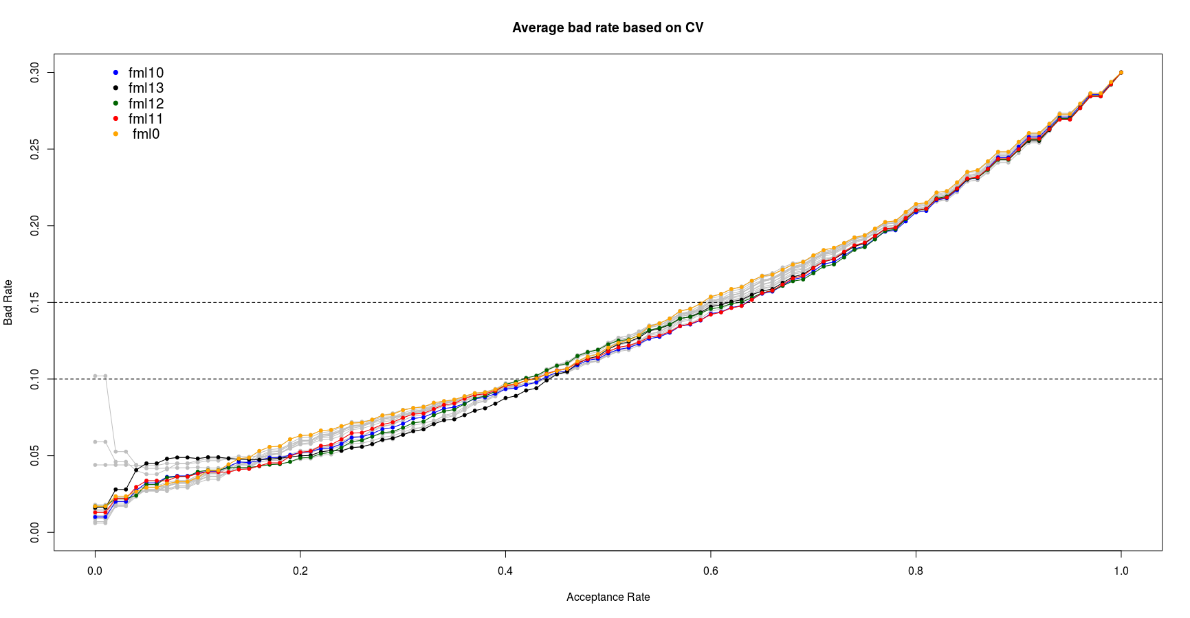
From the above plot we can see the fml10 and fml11 show the best performance in bad rate between 10% to 15%. Since the fml10 has already shown the better AUC I select the fml10 as the best logistic model. It worth note that this model is selected based on the training data set. Its actual performance will be checked in the last section of this report on unseen test data set.
2- Decision Tree
Similar to logistic regression first I split the data to training and test sets.
R> in_train <- createDataPartition(d.g$default, p = 0.66, list = FALSE)
R> train_set <- d.g[in_train,]
R> test_set <- d.g[-in_train,]

R> prop.table(table(train_set$default))
Nondef  Def
 0.7    0.3

R> prop.table(table(test_set$default))
Nondef  Def
 0.7    0.3
I use rpart & rpart.plot packages for applying decision tree algorithm and plotting trees. First I construct the trees with different complexity parameter values and choose the proposed trees based on the minimum average cross-validate error.
R> library(rpart)
R> library(rpart.plot)

R> xerr.matrix <- NULL
R> for ( i in 1:1000)
+ {
+ fml1 <- rpart(default ~ ., method = "class", data = train_set, control = rpart.control(cp = 0.0001))
+ dum <- printcp(fml0)
+ xerr.matrix <- cbind(xerr.matrix, dum[,4])
+ }
R> rownames(xerr.matrix) <- round(dum[,1], digits=6)

R> boxplot(t(xerr.matrix))
R> mean.xerr <- apply(xerr.matrix, 1, mean)
R> points(1:7, mean.xerr, pch=20, col='red', cex=2)
The results are plotted below:
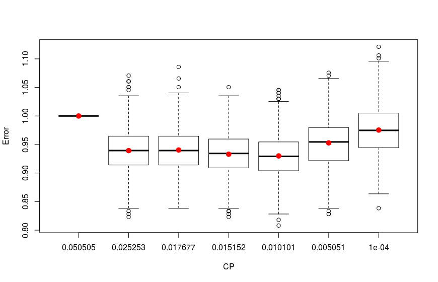
As we see the four trees with 0.01010101, 0.01515152, 0.01767677 and 0.02525253 CP values have the lowest errors. To have a view on this tree I construct and prune trees with these CP values and plot them:
R> id <- which.min(mean.xerr)
R> cp.best.xrr <- dum[id,1] #[1] 0.01010101
R> cp.table.sample <- dum

R> fml2 <- prune(fml0, cp = cp.best.xrr) # 0.01010101
R> fml3 <- prune(fml0, cp = dum[4,1]) # 0.01515152
R> fml4 <- prune(fml0, cp = dum[3,1]) # 0.01767677
R> fml5 <- prune(fml0, cp = dum[2,1]) # 0.02525253
The prp function is used to plot trees:
R> for (i in paste0('fml', 1:5))
+ {
+ png(file=paste0(i,'.png'), width = 1500, height = 800)
+ prp(get(i), main=i)
+ dev.off()
+ }
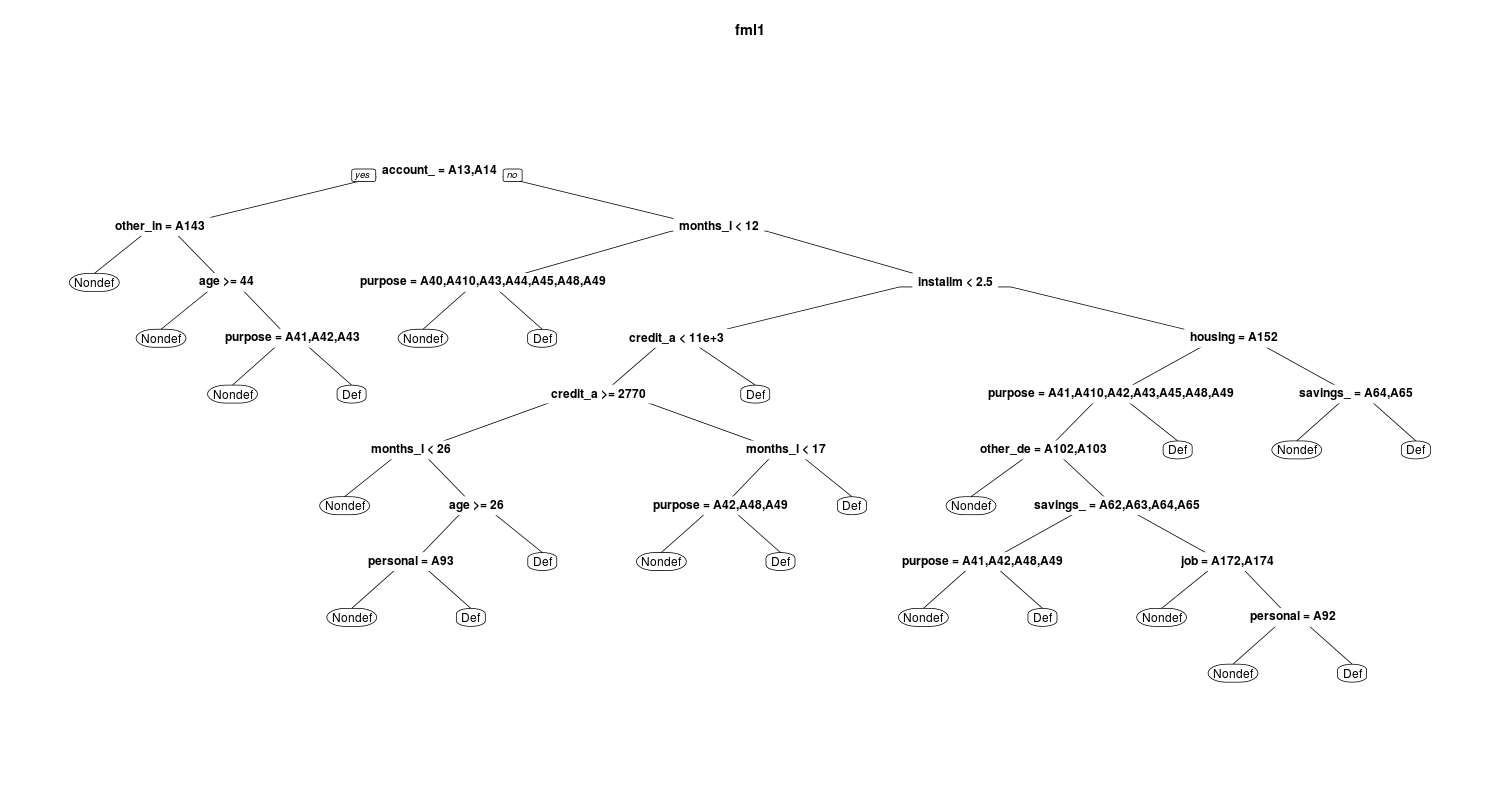
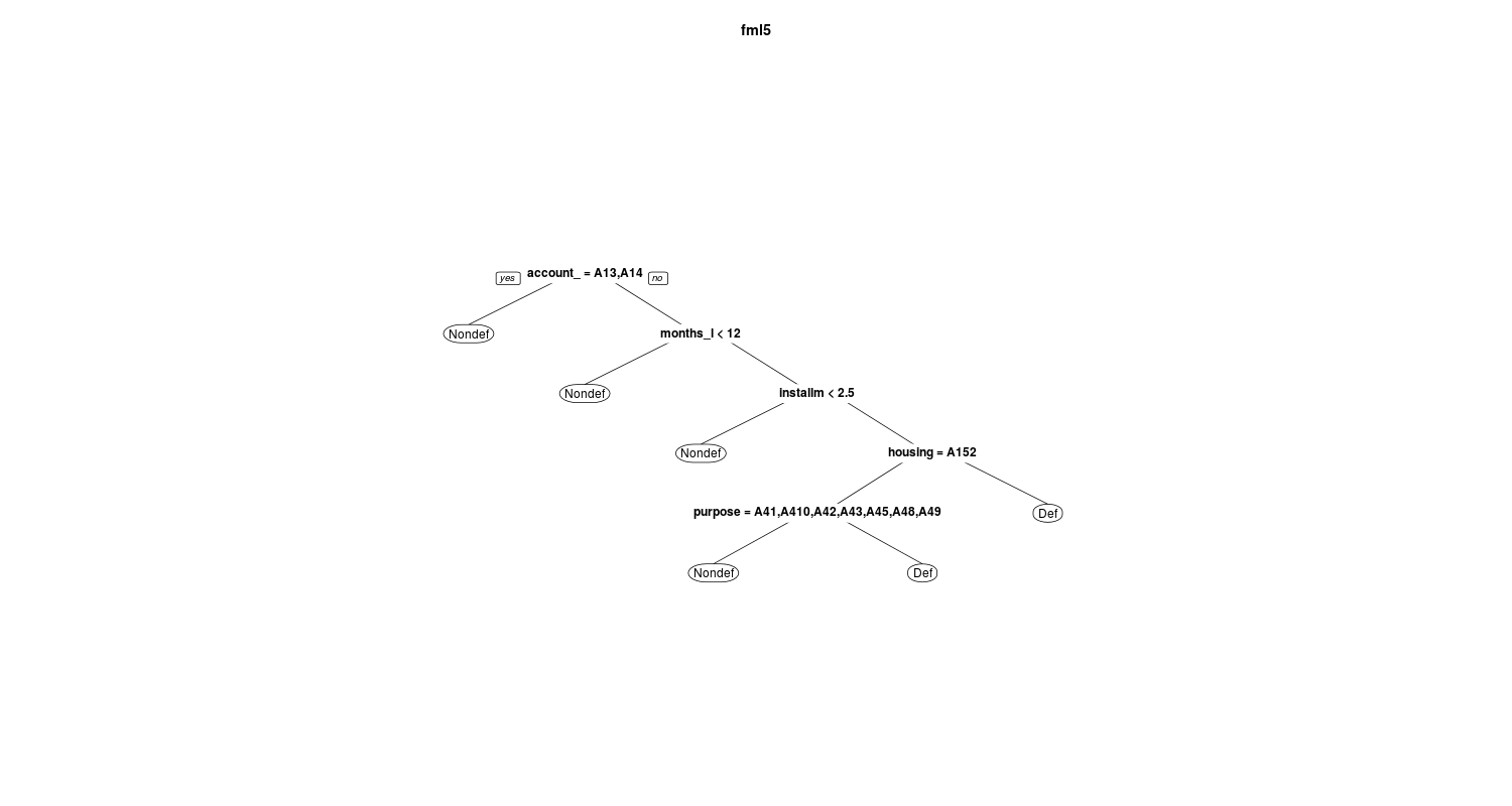
In the below figures you can see and compare the fml1 and fml5:
and
I also select the trees based on the average AUC value using train function in caret package. To speed up the computation I construct a parallel backend using doMC package:
R> library(doMC)
R> registerDoMC(cores = 9)

R> tc <- trainControl(method = "repeatedcv", number = 10, repeats = 100, classProbs = TRUE, summaryFunction=twoClassSummary)
R> rpart.grid <- expand.grid(.cp=c(1e-7,0.0001,0.0004, 0.0005, seq(0.001, 0.03, by=0.001), seq(0.04,0.06, by=0.005)) )
R> train.rpart.rcv <- train(default ~ .,
                                        data=train_set, method="rpart",
                                        trControl=tc, tuneGrid=rpart.grid, metric='ROC')

R> registerDoSEQ()
The below figure shows the result:
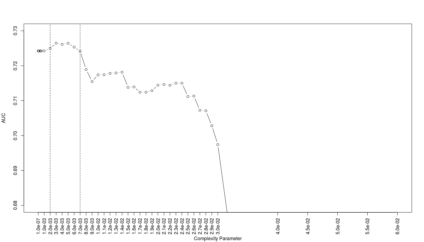
As we can see the trees with CP values between 0.002 to 0.007 show the best AUC efficiency. Totally I have 10 proposed trees with different CP values.
Following the similar procedure in evaluation of logistic models, I evaluate 10 proposed trees based on their bad rate and other statistics through below codes and functions:
#------br.se.ac function--------------------------------------------------
R> br.se.ac <- function(actl_class, pred_prob)
+ {
+ acp_rate <- seq(0,1,by=0.01)
+ cut_off <- NULL
+ bad_rate <- NULL
+ sens <- NULL
+ spec <- NULL
+ accu <- NULL
+ kppa <- NULL
+ for (i in 1:length(acp_rate))
+ {
+ cutoff <- quantile(pred_prob, acp_rate[i])
+ pred_class <- ifelse(pred_prob> cutoff, 'Def', 'Nondef')
+ pred_class <- factor(pred_class, levels=levels(actl_class))

+ cont_table <- table(actl_class, pred_class)

+ TN <- cont_table[1,1]
+ FP <- cont_table[1,2]
+ FN <- cont_table[2,1]
+ TP <- cont_table[2,2]

+ br <- FN/(FN+TN)
+ se <- TP/(TP+FN)
+ sp <- TN/(TN+FP)
+ ac <- (TN+TP)/(TN+FP+FN+TP)


+ py <- ((TP+FN)/(TN+FP+FN+TP)) * ((TP+FP)/(TN+FP+FN+TP))
+ pn <- ((FP+TN)/(TN+FP+FN+TP)) * ((FN+TN)/(TN+FP+FN+TP))
+ pe <- py+pn
+ kp <- (ac-pe)/(1-pe)

+ cut_off <- c(cut_off, cutoff)
+ bad_rate <- c(bad_rate, br)
+ sens <- c(sens, se)
+ spec <- c(spec, sp)
+ accu <- c(accu, ac)
+ kppa <- c(kppa, kp)
+ }
+ data.frame(acp_rate, cut_off, bad_rate, sens, spec, accu, kppa)
+ }

#----cv_br_function ------------------------------------------------------------
R> cv_br_function <- function(cp_par, folds)
+ {
+  br_r <- lapply(folds, function(x)
+  {
+    train_set_train <- train_set[-x, ]
+    train_set_test <- train_set[x, ]
+    mdl         <- rpart(default ~ ., method = "class", data =  train_set_train, control = rpart.control(cp = cp_par))
+    pred        <- predict(mdl, newdata = train_set_test,  type='prob')
+    dum <- br.se.ac(train_set_test$default, pred[,2] )
+    return(dum$bad_rate)
+  })
+  br.matrix <- matrix(unlist(br_r),  ncol=10  )
+  colnames(br.matrix) <- c(paste0('Fold0',1:9),'Fold10')
+  rownames(br.matrix) <- paste0(0:100,'%')
+  return(br.matrix)
+ }

#....Calculating average bad rate for each tree via repeated CV...........
R> n.cv <- 100
R> cp_vec <- c( seq(0.002, 0.007, by=0.001), 0.01010101, 0.01515152, 0.01767677, 0.02525253)
R> for (cp_p in cp_vec)
+ {
+  print(cp_p)
+  t.mat <- NULL
+  for ( j in 1:n.cv)
+  {

+   folds.new <- createFolds(train_set$default, k = 10)
+   dum <- cv_br_function(cp_p, folds.new)
+   t.mat <- cbind(t.mat, dum)
+  }

+  dum2 <- apply(t.mat, 1, mean)
+  dum3 <- paste0('fml_cp_',cp_p,'_br.cv') # e.g. "fml_cp_0.002_br.cv"
+  assign(dum3, dum2)
+ }

#..................plotting...................
plot(seq(0,1,by=0.01), rep(0, 101), type='n', ylim=c(0,0.3), xlab='Acceptance Rate', ylab='Bad Rate', main='Average bad rate based on CV')
for (cp_p in cp_vec)
{
 dum3 <- paste0('fml_cp_',cp_p,'_br.cv') # "fml_cp_0.002_br.cv"
 lines(seq(0,1,by=0.01), get(dum3), type='o', col='grey', pch=20)
}
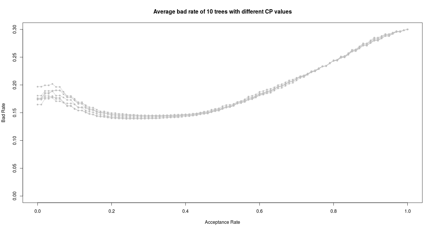
We can see the high bad rate of all 10 proposed trees. In the next section I employ and train the random forest algorithm on the data.
3. Random Forest
Using caret package I train random forest on training data set considering AUC for different mtry values (number of features which are randomly selected at each split) in a repeated cross-validation method. I also use a parallel backend to speed up the computation.
library(caret)
library(doMC)
registerDoMC(cores = 12)

tc <- trainControl(method = "repeatedcv", number = 10, repeats = 100, classProbs = TRUE, summaryFunction=twoClassSummary)
rf_grid <- expand.grid(.mtry = c(2, 3, 4, 5, 6, 7, 8, 9, 10, 16, 20))
m_rf <- train(default ~ ., data = train_set, method = "rf", metric = "ROC", trControl = tc, tuneGrid = rf_grid)

registerDoSEQ()
I plot the results as below:
plot(m_rf$results$mtry, m_rf$results$ROC, typ='b', xaxt='n', xlab='mtry', ylab='AUC')
axis(1,at= c(2, 3, 4, 5, 6, 7, 8, 9, 10, 16, 20) , las=2,col.axis='black',col='black')
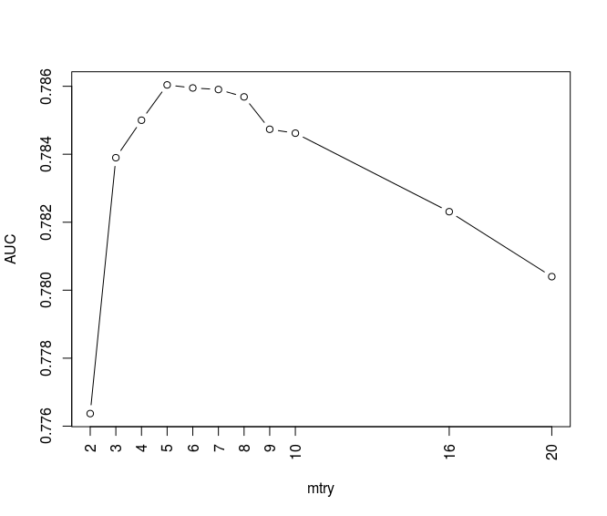
We can see the random forest corresponding to mtry values between 3 to 10 shows high values in AUC. Using br.se.ac function in previous section and below codes and functions I calculate the bad rate all proposed random forest models:
#----Evaluating and plotting of bad rate vs acceptance rate of all *RANDOM FOREST* models bulit on CV---------------------------------------------------
R> cv_br_function_rf <- function(mtry_par, folds)
+ {
+  br_r <- lapply(folds, function(x)
+  {
+   train_set_train <- train_set[-x, ]
+   train_set_test <- train_set[x, ]
+   mdl <- randomForest(default ~ ., data = train_set_train, ntree=500, mtry=mtry_par)
+   pred        <- predict(mdl, newdata=train_set_test, type = 'prob')
+   dum <- br.se.ac(train_set_test$default, pred[,2] )

+   return(dum$bad_rate)
+  })
+ br.matrix <- matrix(unlist(br_r),  ncol=10  )
+ colnames(br.matrix) <- c(paste0('Fold0',1:9),'Fold10')
+ rownames(br.matrix) <- paste0(0:100,'%')

+ return(br.matrix)
+}

#....Calculating average bad rate for each model via CV...........
R> library(randomForest)
R> n.cv <- 100
R> mtry_vec <- 3:10

R> for (mtry_p in mtry_vec)
+ {
+  t.mat <- NULL
+  for ( j in 1:n.cv)
+  {
+   folds.new <- createFolds(train_set$default, k = 10)
+   dum <- cv_br_function_rf(mtry_p, folds.new)
+   t.mat <- cbind(t.mat, dum)
+  }

+  dum2 <- apply(t.mat, 1, mean)
+  dum3 <- paste0('fml_mtry_',mtry_p,'_br.cv') # e.g. "fml_mtry_3_br.cv"
+  assign(dum3, dum2)
+ }
The results are plotted:
R> plot(seq(0,1,by=0.01), rep(0, 101), type='n', ylim=c(0,0.3), xlab='Acceptance Rate', ylab='Bad Rate', main='Average bad rate of 10 trees (gold color) and 8 random forest models (grey)')
R> for (cp_p in cp_vec)
+  {
+   dum3 <- paste0('fml_cp_',cp_p,'_br.cv') # e.g. "fml_cp_0.002_br.cv"
+   lines(seq(0,1,by=0.01), get(dum3), type='o', col='lightgoldenrod', pch=20)
+  }
R> for (mtry_p in mtry_vec)
+  {
+   dum3 <- paste0('fml_mtry_',mtry_p,'_br.cv') # e.g. "fml_mtry_10_br.cv"
+   lines(seq(0,1,by=0.01), get(dum3), type='o', col='grey', pch=20)
+  }

R> lines(seq(0,1,by=0.01), fml_mtry_3_br.cv, type='o', col='red', pch=20)
R> abline(h=0.1, lty=2)
R> abline(h=0.15, lty=2)
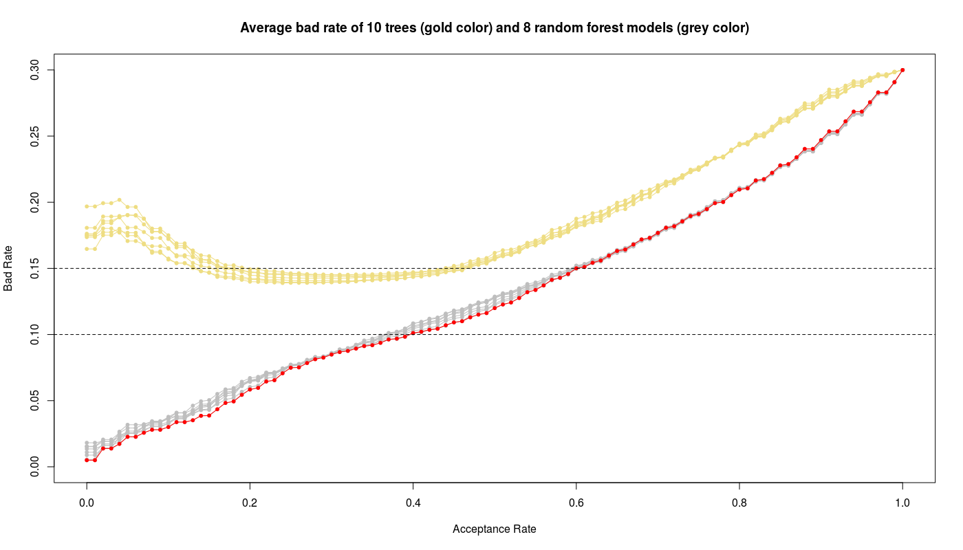
In above figure I have also plotted the results of trees (gold color) to compare with random forest models (gray color). We see obviously the random forest models work better than trees while the random forest with mtry=3 gives the best performance i.e. low bad rate and high acceptance rate.
Results of the final models
The fml10 logistic model and random forest with mtry=3 are the winners on training data set. To see the real performance of both models I test them on unseen test data set. The logistic fml10 model can evaluate via using br.se.ac function defined in logistic section as:
mdl <- glm(formula = fml10, family = binomial(link=logit), data = train_set)
pred      <- predict(mdl, newdata = test_set, type = 'response')
log_fml10_results <- br.se.ac(test_set$default, pred )
Since random forest has the randomness inherent I calculate a average of performance of the model with mtry=3:
R> sum_mat <- matrix(0, nrow=101,ncol=7)
R> for (i in 1:100)
+  {
+   mdl <- randomForest(default ~ ., data = train_set, ntree=500, mtry=3)
+   pred <- predict(mdl, newdata=test_set, type = 'prob')
+   dum <- br.se.ac(test_set$default, pred[,2] )
+   sum_mat <- sum_mat + dum
+  }

R> rf_mtry3_results <- sum_mat/100
Assuming maximum 15% bad rate we have:
acp_rate    cut_off   bad_rate    sens       spec        accu      kppa
Logistic Regression
65% 0.65 0.44823798 0.14932127 0.67647059 0.789915966 0.7558824 0.445187166

Random Forest
63% 0.63 0.4042546 0.151472427 0.68137255 0.764957983 0.7398824 0.418835806
The below figure illustrates the bad rate for both models:
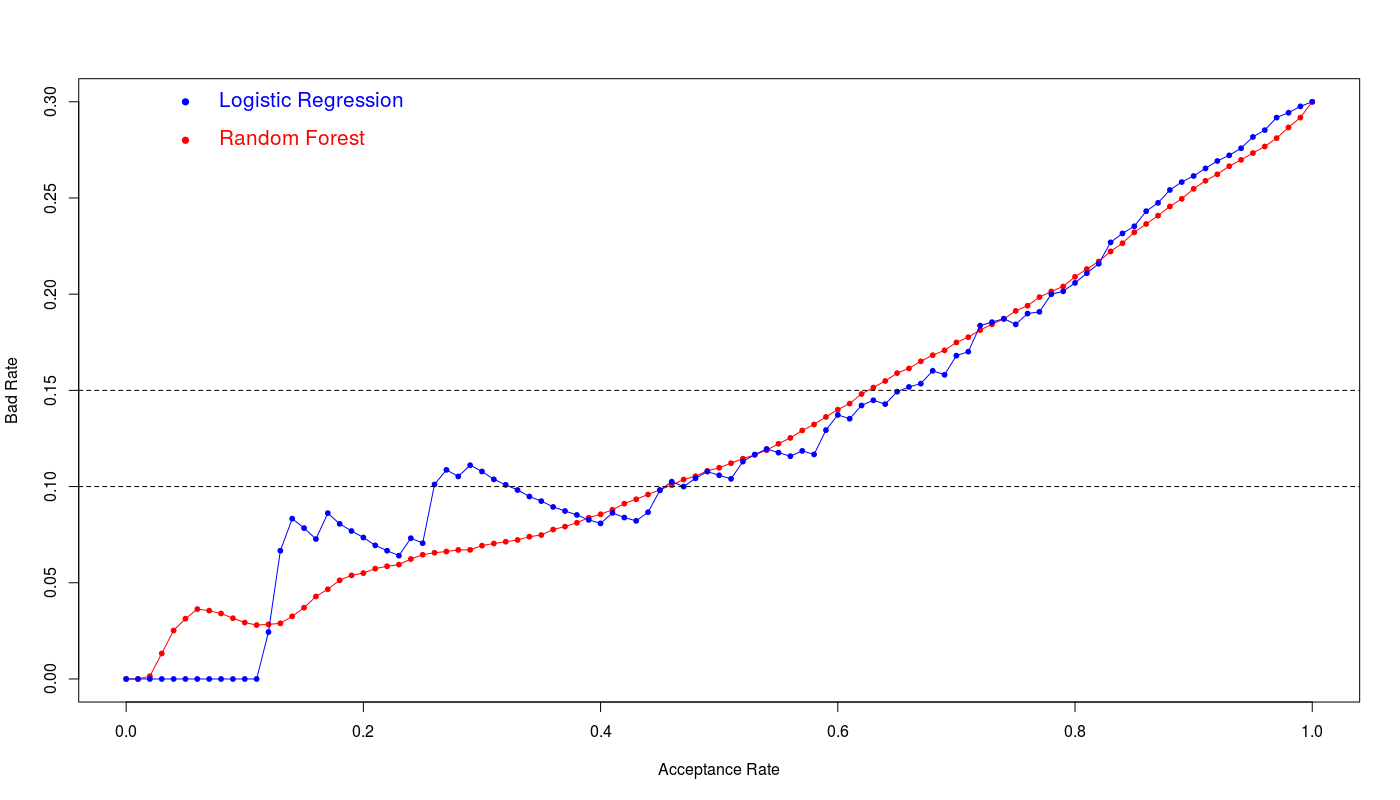
We see the logistic regression and random forest show the similar efficiency however logistic regression shows slightly better performance at 15% bad rate. The 65% acceptance ratio at 15% bad rate with 76% accuracy and 0.44 kappa value is a good achievement for this model.